Choose the best data source for your Amazon SageMaker training job

Amazon SageMaker is a managed service that makes it easy to build, train, and deploy machine learning (ML) models. Data scientists use SageMaker training jobs to easily train ML models; you don’t have to worry about managing compute resources, and you pay only for the actual training time. Data ingestion is an integral part of any training pipeline, and SageMaker training jobs support a variety of data storage and input modes to suit a wide range of training workloads.

This post helps you choose the best data source for your SageMaker ML training use case. We introduce the data sources options that SageMaker training jobs support natively. For each data source and input mode, we outline its ease of use, performance characteristics, cost, and limitations. To help you get started quickly, we provide the diagram with a sample decision flow that you can follow based on your key workload characteristics. Lastly, we perform several benchmarks for realistic training scenarios to demonstrate the practical implications on the overall training cost and performance.

Native SageMaker data sources and input modes

Reading training data easily and flexibly in a performant way is a common recurring concern for ML training. SageMaker simplifies data ingestion with a selection of efficient, high-throughput data ingestion mechanisms called data sources and their respective input modes. This allows you to decouple training code from the actual data source, automatically mount file systems, read with high performance, easily turn on data sharding between GPUs and instances to enable data parallelism, and auto shuffle data at the start of each epoch.

The SageMaker training ingestion mechanism natively integrates with three AWS managed storage services:

• Amazon Simple Storage Service (Amazon S3) is an object storage service that offers industry-leading scalability, data availability, security, and performance.
• Amazon FSx for Lustre is a fully managed shared storage with the scalability and performance of the popular Lustre file system. It’s usually linked to an existing S3 bucket.
• Amazon Elastic File System (Amazon EFS) is a general purpose, scalable, and highly available shared file system with multiple price tiers. Amazon EFS is serverless and automatically grows and shrinks as you add and remove files.

SageMaker training allows your training script to access datasets stored on Amazon S3, FSx for Lustre, or Amazon EFS, as if it were available on a local file system (via a POSIX-compliant file system interface).

With Amazon S3 as a data source, you can choose between File mode, FastFile mode, and Pipe mode:

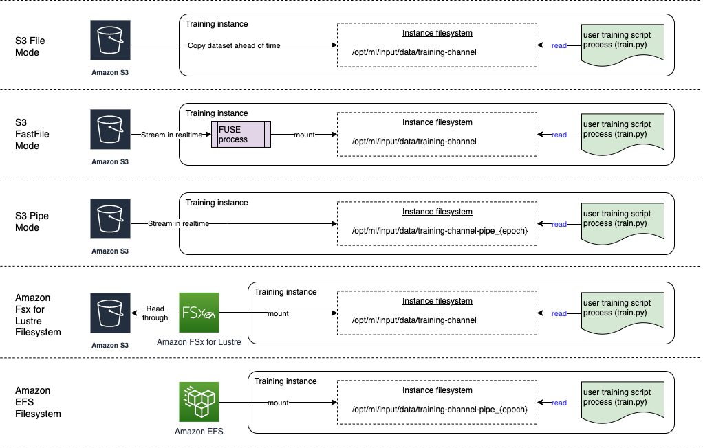
• File mode – SageMaker copies a dataset from Amazon S3 to the ML instance storage, which is an attached Amazon Elastic Block Store (Amazon EBS) volume or NVMe SSD volume, before your training script starts.
• FastFile mode – SageMaker exposes a dataset residing in Amazon S3 as a POSIX file system on the training instance. Dataset files are streamed from Amazon S3 on demand as your training script reads them.
• Pipe mode – SageMaker streams a dataset residing in Amazon S3 to the ML training instance as a Unix pipe, which streams from Amazon S3 on demand as your training script reads the data from the pipe.

With FSx for Lustre or Amazon EFS as a data source, SageMaker mounts the file system before your training script starts.

Training input channels

When launching an SageMaker training job, you can specify up to 20 managed training input channels. You can think of channels as an abstraction unit to tell the training job how and where to get the data that is made available to the algorithm code to read from a file system path (for example, /opt/ml/input/data/input-channel-name) on the ML instance. The selected training channels are captured as part of the training job metadata in order to enable a full model lineage tracking for use cases such as reproducibility of training jobs or model governance purposes.

To use Amazon S3 as your data source, you define a TrainingInput to specify the following:

• Your input mode (File, FastFile, or Pipe mode)
• Distribution and shuffling configuration
• An S3DataType as one of three methods for specifying objects in Amazon S3 that make up your dataset:
  • S3Prefix (all objects under the S3 prefix)
  • Manifest file (a list of S3 objects)
  • Augmented manifest file (a list of S3 objects and their respective labels)

Alternatively, for FSx for Lustre or Amazon EFS, you define a FileSystemInput.

The following diagram shows five training jobs, each configured with a different data source and input mode combination:

Data sources and input modes

The follow sections provide a deep dive into the differences between Amazon S3 (File mode, FastFile mode, and Pipe mode), FSx for Lustre, and Amazon EFS as SageMaker ingestion mechanisms.

Amazon S3 File mode

File mode is the default input mode (if you didn’t explicitly specify one), and it’s the more straightforward to use. When you use this input option, SageMaker downloads the dataset from Amazon S3 into the ML training instance storage (Amazon EBS or local NVMe depending on the instance type) on your behalf before launching model training, so that the training script can read the dataset from the local file system. In this case, the instance must have enough storage space to fit the entire dataset.

You configure the dataset for File mode by providing either an S3 prefix, manifest file, or augmented manifest file.

You should use an S3 prefix when all your dataset files are located within a common S3 prefix (subfolders are okay).

The manifest file lists the files comprising your dataset. You typically use a manifest when a data preprocessing job emits a manifest file, or when your dataset files are spread across multiple S3 prefixes. An augmented manifest is a JSON line file, where each line contains a list of attributes, such as a reference to a file in Amazon S3, alongside additional attributes, mostly labels. Its use cases are similar to that of a manifest.

File mode is compatible with SageMaker local mode (starting a SageMaker training container interactively in seconds). For distributed training, you can shard the dataset across multiple instances with the ShardedByS3Key option.

File mode download speed depends on dataset size, average file size, and number of files. For example, the larger the dataset is (or the more files it has), the longer the downloading stage is, during which the compute resource of the instance remains effectively idle. When training with Spot Instances, the dataset is downloaded each time the job resumes after a Spot interruption. Typically, data downloading takes place at approximately 200 MB/s for large files (for example, 5 minutes/50 GB). Whether this startup overhead is acceptable primarily depends on the overall duration of your training job, because a longer training phase means a proportionally smaller download phase.

Amazon S3 FastFile mode

FastFile mode exposes S3 objects via a POSIX-compliant file system interface, as if the files were available on the local disk of your training instance, and streams their content on demand when data is consumed by the training script. This means your dataset no longer needs to fit into the training instance storage space, and you don’t need to wait for the dataset to be downloaded to the training instance before training can start.

To facilitate this, SageMaker lists all the object metadata stored under the specified S3 prefix before your training script runs. This metadata is used to create a read-only FUSE (file system in userspace) that is available to your training script via /opt/ml/data/training-channel-name. Listing S3 objects runs as fast as 5,500 objects per seconds regardless of their size. This is much quicker than downloading files upfront, as is the case with File mode. While your training script is running, it can list or read files as if they were available locally. Each read operation is delegated to the FUSE service, which proxies GET requests to Amazon S3 in order to deliver the actual file content to the caller. Like a local file system, FastFile treats files as bytes, so it’s agnostic to file formats. FastFile mode can reach a throughput of more than one GB/s when reading large files sequentially using multiple workers. You can use FastFile to read small files or retrieve random byte ranges, but you should expect a lower throughput for such access patterns. You can optimize your read access pattern by serializing many small files into larger file containers, and read them sequentially.

FastFile currently supports S3 prefixes only (no support for manifest and augmented manifest), and FastFile mode is compatible with SageMaker local mode.

Amazon S3 Pipe mode

Pipe mode is another streaming mode that is largely replaced by the newer and simpler-to-use FastFile mode.

With Pipe mode, data is pre-fetched from Amazon S3 at high concurrency and throughput, and streamed into Unix named FIFO pipes. Each pipe may only be read by a single process. A SageMaker-specific extension to TensorFlow conveniently integrates Pipe mode into the native TensorFlow data loader for streaming text, TFRecords, or RecordIO file formats. Pipe mode also supports managed sharding and shuffling of data.

FSx for Lustre

FSx for Lustre can scale to hundreds of GB/s of throughput and millions of IOPS with low-latency file retrieval.

When starting a training job, SageMaker mounts the FSx for Lustre file system to the training instance file system, then starts your training script. Mounting itself is a relatively fast operation that doesn’t depend on the size of the dataset stored in FSx for Lustre.

In many cases, you create an FSx for Lustre file system and link it to an S3 bucket and prefix. When linked to a S3 bucket as source, files are lazy-loaded into the file system as your training script reads them. This means that right after the first epoch of your first training run, the entire dataset is copied from Amazon S3 to the FSx for Lustre storage (assuming an epoch is defined as a single full sweep thought the training examples, and that the allocated FSx for Lustre storage is large enough). This enables low-latency file access for any subsequent epochs and training jobs with the same dataset.

You can also preload files into the file system before starting the training job, which alleviates the cold start due to lazy loading. It’s also possible to run multiple training jobs in parallel that are serviced by the same FSx for Lustre file system. To access FSx for Lustre, your training job must connect to a VPC (see VPCConfig settings), which requires DevOps setup and involvement. To avoid data transfer costs, the file system uses a single Availability Zone, and you need to specify this Availability Zone ID when running the training job. Because you’re using Amazon S3 as your long-term data storage, we recommend deploying your FSx for Lustre with Scratch 2 storage, as a cost-effective, short-term storage choice for high throughput, providing a baseline of 200 MB/s and a burst of up to 1300 MB/s per TB of provisioned storage.

With your FSx for Lustre file system constantly running, you can start new training jobs without waiting for a file system to be created, and don’t have to worry about the cold start during the very first epoch (because files could still be cached in the FSx for Lustre file system). The downside in this scenario is the extra cost associated with keeping the file system running. Alternatively, you could create and delete the file system before and after each training job (probably with scripted automation to help), but it takes time to initialize an FSx for Lustre file system, which is proportional to the number of files it holds (for example, it takes about an hour to index approximately 2 million objects from Amazon S3).

Amazon EFS

We recommend using Amazon EFS if your training data already resides in Amazon EFS due to use cases besides ML training. To use Amazon EFS as a data source, the data must already reside in Amazon EFS prior to training. SageMaker mounts the specified Amazon EFS file system to the training instance, then starts your training script. When configuring the Amazon EFS file system, you need to choose between the default General Purpose performance mode, which is optimized for latency (good for small files), and Max I/O performance mode, which can scale to higher levels of aggregate throughput and operations per second (better for training jobs with many I/O workers). To learn more, refer to Using the right performance mode.

Additionally, you can choose between two metered throughput options: bursting throughput, and provisioned throughput. Bursting throughput for a 1 TB file system provides a baseline of 150 MB/s, while being able to burst to 300 MB/s for a time period of 12 hours a day. If you need higher baseline throughput, or find yourself running out of burst credits too many times, you could either increase the size of the file system or switch to provisioned throughput. In provisioned throughput, you pay for the desired baseline throughput up to a maximum of 3072 MB/s read.

Your training job must connect to a VPC (see VPCConfig settings) to access Amazon EFS.

Choosing the best data source

The best data source for your training job depends on workload characteristics like dataset size, file format, average file size, training duration, sequential or random data loader read pattern, and how fast your model can consume the training data.

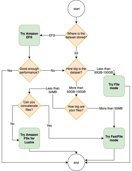
The following flowchart provides some guidelines to help you get started:

When to use Amazon EFS

If your dataset is primarily stored on Amazon EFS, you may have a preprocessing or annotations application that uses Amazon EFS for storage. You could easily run a training job configured with a data channel that points to the Amazon EFS file system (for more information, refer to Speed up training on Amazon SageMaker using Amazon FSx for Lustre and Amazon EFS file systems). If performance is not quite as good as you expected, check your optimization options with the Amazon EFS performance guide, or consider other input modes.

Use File mode for small datasets

If the dataset is stored on Amazon S3 and its overall volume is relatively small (for example, less than 50–100 GB), try using File mode. The overhead of downloading a dataset of 50 GB can vary based on the total number of files (for example, about 5 minutes if chunked into 100 MB shards). Whether this startup overhead is acceptable primarily depends on the overall duration of your training job, because a longer training phase means a proportionally smaller download phase.

Serializing many small files together

If your dataset size is small (less than 50–100 GB), but is made up of many small files (less than 50 MB), the File mode download overhead grows, because each file needs to be downloaded individually from Amazon S3 to the training instance volume. To reduce this overhead, and to speed up data traversal in general, consider serializing groups of smaller files into fewer larger file containers (such as 150 MB per file) by using file formats such as TFRecord for TensorFlow, WebDataset for PyTorch, or RecordIO for MXNet. These formats require your data loader to iterate through examples sequentially. You could still shuffle your data by randomly reordering the list of TFRecord files after each epoch, and by randomly sampling data from a local shuffle buffer (see the following TensorFlow example).

When to use FastFile mode

For larger datasets with larger files (more than 50 MB), the first option is to try FastFile mode, which is more straightforward to use than FSx for Lustre because it doesn’t require creating a file system, or connecting to a VPC. FastFile mode is ideal for large file containers (more than 150 MB), and might also do well with files more than 50 MB. Because FastFile mode provides a POSIX interface, it supports random reads (reading non-sequential byte-ranges). However, this isn’t the ideal use case, and your throughput would probably be lower than with the sequential reads. However, if you have a relatively large and computationally intensive ML model, FastFile mode may still be able to saturate the effective bandwidth of the training pipeline and not result in an I/O bottleneck. You’ll need to experiment and see. Luckily, switching from File mode to FastFile (and back) is as easy as adding (or removing) the input_mode='FastFile' parameter while defining your input channel using the SageMaker Python SDK:

sagemaker.inputs.TrainingInput(S3_INPUT_FOLDER, input_mode='FastFile') 

No other code or configuration needs to change.

When to use FSx for Lustre

If your dataset is too large for File mode, or has many small files (which you can’t serialize easily), or you have a random read access pattern, FSx for Lustre is a good option to consider. Its file system scales to hundreds of GB/s of throughput and millions of IOPS, which is ideal when you have many small files. However, as already discussed earlier, be mindful of the cold start issues due to lazy loading, and the overhead of setting up and initializing the FSx for Lustre file system.

Cost considerations

For the majority of ML training jobs, especially jobs utilizing GPUs or purpose-built ML chips, most of the cost to train is the ML training instance’s billable seconds. Storage GB per month, API requests, and provisioned throughput are additional costs that are directly associated with the data sources you use.

Storage GB per month

Storage GB per month can be significant for larger datasets, such as videos, LiDAR sensor data, and AdTech real-time bidding logs. For example, storing 1 TB in the Amazon S3 Intelligent-Tiering Frequent Access Tier costs $23 per month. Adding the FSx for Lustre file system on top of Amazon S3 results in additional costs. For example, creating a 1.2 TB file system of SSD-backed Scratch 2 type with data compression disabled costs an additional $168 per month ($140/TB/month).

With Amazon S3 and Amazon EFS, you pay only for what you use, meaning that you’re charged according to the actual dataset size. With FSx for Lustre, you’re charged by the provisioned file system size (1.2 TB at minimum). When running ML instances with EBS volumes, Amazon EBS is charged independently of the ML instance. This is usually a much lower cost compared to the cost of running the instance. For example, running an ml.p3.2xlarge instance with a 100 GB EBS volume for 1 hour costs $3.825 for the instance and $0.02 for the EBS volume.

API requests and provisioned throughput cost

While your training job is crunching through the dataset, it lists and fetches files by dispatching Amazon S3 API requests. For example, each million GET requests is priced at $0.4 (with the Intelligent-Tiering class). You should expect no data transfer cost for bandwidth in and out of Amazon S3, because training takes place in a single Availability Zone.

When using an FSx for Lustre that is linked to an S3 bucket, you incur Amazon S3 API request costs for reading data that isn’t yet cached in the file system, because FSx For Lustre proxies the request to Amazon S3 (and caches the result). There are no direct request costs for FSx for Lustre itself. When you use an FSx for Lustre file system, avoid costs for cross-Availability Zone data transfer by running your training job connected to the same Availability Zone that you provisioned the file system in. Amazon EFS with provisioned throughput adds an extra cost to consdier beyond GB per month.

Performance case study

To demonstrate the training performance considerations mentioned earlier, we performed a series of benchmarks for a realistic use case in the computer vision domain. The benchmark (and takeaways) from this section might not be applicable to all scenarios, and are affected by various predetermined factors we used, such as DNN. We ran tests for 12 combinations of the following:

• Input modes – FSx for Lustre, File mode, FastFile mode
• Dataset size – Smaller dataset (1 GB), larger dataset (54 GB)
• File size – Smaller files (JPGs, approximately 39 KB), Larger files (TFRecord, approximately 110 MB)

For this case study, we chose the most widely used input modes, and therefore omitted Amazon EFS and Pipe mode.

The case study benchmarks were designed as end-to-end SageMaker TensorFlow training jobs on an ml.p3.2xlarge single-GPU instance. We chose the renowned ResNet-50 as our backbone model for the classification task and Caltech-256 as the smaller training dataset (which we replicated 50 times to create its larger dataset version). We performed the training for one epoch, defined as a single full sweep thought the training examples.

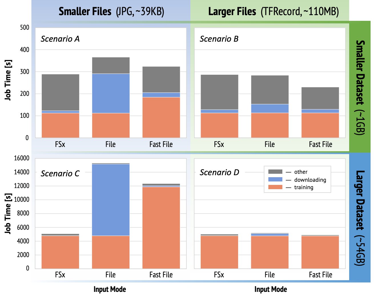
The following graphs show the total billable time of the SageMaker training jobs for each benchmark scenario. The total job time itself is comprised of downloading, training, and other stages (such as container startup and uploading trained model artifacts to Amazon S3). Shorter billable times translate into faster and cheaper training jobs.

Let’s first discuss Scenario A and Scenario C, which conveniently demonstrate the performance difference between input modes when the dataset is comprised of many small files.

Scenario A (smaller files, smaller dataset) reveals that the training job with the FSx for Lustre file system has the smallest billable time. It has the shortest downloading phase, and its training stage is as fast as File mode, but faster than FastFile. FSx for Lustre is the winner in this single epoch test. Having said that, consider a similar workload but with multiple epochs—the relative overhead of File mode due to the downloading stage decreases as more epochs are added. In this case, we prefer File mode for its ease of use. Additionally, you might find that using File mode and paying for 100 extra billable seconds is a better choice than paying for and provisioning an FSx for Lustre file system.

Scenario C (smaller files, larger dataset) shows FSx for Lustre as the fastest mode, with only 5,000 seconds of total billable time. It also has the shortest downloading stage, because mounting the FSx for Lustre file system doesn’t depend on the number of files in the file system (1.5 million files in this case). The downloading overhead of FastFile is also small; it only fetches metadata of the files residing under the specified S3 bucket prefix, while the content of the files is read during the training stage. File mode is the slowest mode, spending 10,000 seconds to download the entire dataset upfront before starting training. When we look at the training stage, FSx for Lustre and File mode demonstrate similar excellent performance. As for FastFile mode, when streaming smaller files directly from Amazon S3, the overhead for dispatching a new GET request for each file becomes significant relative to the total duration of the file transfer (despite using a highly parallel data loader with prefetch buffer). This results in an overall lower throughput for FastFile mode, which creates an I/O bottleneck for the training job. FSx for Lustre is the clear winner in this scenario.

Scenarios B and D show the performance difference across input modes when the dataset is comprised of fewer larger files. Reading sequentially using larger files typically results in better I/O performance because it allows effective buffering and reduces the number of I/O operations.

Scenario B (larger files, smaller dataset) shows similar training stage time for all modes (testifying that the training isn’t I/O-bound). In this scenario, we prefer FastFile mode over File mode due to shorter downloading stage, and prefer FastFile mode over FSx for Lustre due to the ease of use of the former.

Scenario D (larger files, larger dataset) shows relatively similar total billable times for all three modes. The downloading phase of File mode is longer than that of FSx for Lustre and FastFile. File mode downloads the entire dataset (54 GB) from Amazon S3 to the training instance before starting the training stage. All three modes spend similar time in the training phase, because all modes can fetch data fast enough and are GPU-bound. If we use ML instances with additional CPU or GPU resources, such as ml.p4d.24xlarge, the required data I/O throughput to saturate the compute resources grows. In these cases, we can expect FastFile and FSx for Lustre to successfully scale their throughput (however, FSx for Lustre throughput depends on provisioned file system size). The ability of File mode to scale its throughput depends on the throughput of the disk volume attached to the instance. For example, Amazon EBS-backed instances (like ml.p3.2xlarge, ml.p3.8xlarge, and ml.p3.16xlarge) are limited to a maximum throughput of 250MB/s, whereas local NVMe-backed instances (like ml.g5.* or ml.p4d.24xlarge) can accommodate a much larger throughput.

To summarize, we believe FastFile is the winner for this scenario because it’s faster than File mode, and just as fast as FSx for Lustre, yet more straightforward to use, costs less, and can easily scale up its throughput as needed.

Additionally, if we had a much larger dataset (several TBs in size), File mode would spend many hours downloading the dataset before training could start, whereas FastFile could start training significantly more quickly.

Bring your own data ingestion

The native data source of SageMaker fits most but not all possible ML training scenarios. The situations when you might need to look for other data ingestion options could include reading data directly from a third-party storage product (assuming an easy and timely export to Amazon S3 isn’t possible), or having a strong requirement for the same training script to run unchanged on both SageMaker and Amazon Elastic Compute Cloud (Amazon EC2) or Amazon Elastic Kubernetes Service (Amazon EKS). You can address these cases by implementing your data ingestion mechanism into the training script. This mechanism is responsible for reading datasets from external data sources into the training instance. For example, the TFRecordDataset of the TensorFlow’s tf.data library can read directly from Amazon S3 storage.

If your data ingestion mechanism needs to call any AWS services, such as Amazon Relational Database Service (Amazon RDS), make sure that the AWS Identity and Access Management (IAM) role of your training job includes the relevant IAM policies. If the data source resides in Amazon Virtual Private Cloud (Amazon VPC), you need to run your training job connected to the same VPC.

When you’re managing dataset ingestion yourself, SageMaker lineage tracking can’t automatically log the datasets used during training. Therefore, consider alternative mechanisms, like training job tags or hyperparameters, to capture your relevant metadata.

Conclusion

Choosing the right SageMaker training data source could have a profound effect on the speed, ease of use, and cost of training ML models. Use the provided flowchart to get started quickly, observe the results, and experiment with additional configuration as needed. Keep in mind the pros, cons, and limitations of each data source, and how well they suit your training job’s individual requirements. Reach out to an AWS contact for further information and assistance.

About the Authors

Gili Nachum is a senior AI/ML Specialist Solutions Architect who works as part of the EMEA Amazon Machine Learning team. Gili is passionate about the challenges of training deep learning models, and how machine learning is changing the world as we know it. In his spare time, Gili enjoy playing table tennis.

Dr. Alexander Arzhanov is an AI/ML Specialist Solutions Architect based in Frankfurt, Germany. He helps AWS customers to design and deploy their ML solutions across EMEA region. Prior to joining AWS, Alexander was researching origins of heavy elements in our universe and grew passionate about ML after using it in his large-scale scientific calculations.

• Coinsmart. Europe’s Best Bitcoin and Crypto Exchange.
• Platoblockchain. Web3 Metaverse Intelligence. Knowledge Amplified. FREE ACCESS.
• CryptoHawk. Altcoin Radar. Free Trial.
• Source: https://aws.amazon.com/blogs/machine-learning/choose-the-best-data-source-for-your-amazon-sagemaker-training-job/