The Batch Normalization layer of Keras is broken

• April 17, 2018
• Vasilis Vryniotis
• . 30 Comments

UPDATE: Unfortunately my Pull-Request to Keras that changed the behaviour of the Batch Normalization layer was not accepted. You can read the details here. For those of you who are brave enough to mess with custom implementations, you can find the code in my branch. I might maintain it and merge it with the latest stable version of Keras (2.1.6, 2.2.2 and 2.2.4) for as long as I use it but no promises.

Most people who work in Deep Learning have either used or heard of Keras. For those of you who haven’t, it’s a great library that abstracts the underlying Deep Learning frameworks such as TensorFlow, Theano and CNTK and provides a high-level API for training ANNs. It is easy to use, enables fast prototyping and has a friendly active community. I’ve been using it heavily and contributing to the project periodically for quite some time and I definitely recommend it to anyone who wants to work on Deep Learning.

Even though Keras made my life easier, quite many times I’ve been bitten by the odd behavior of the Batch Normalization layer. Its default behavior has changed over time, nevertheless it still causes problems to many users and as a result there are several related open issues on Github. In this blog post, I will try to build a case for why Keras’ BatchNormalization layer does not play nice with Transfer Learning, I’ll provide the code that fixes the problem and I will give examples with the results of the patch.

On the subsections below, I provide an introduction on how Transfer Learning is used in Deep Learning, what is the Batch Normalization layer, how learnining_phase works and how Keras changed the BN behavior over time. If you already know these, you can safely jump directly to section 2.

1.1 Using Transfer Learning is crucial for Deep Learning

One of the reasons why Deep Learning was criticized in the past is that it requires too much data. This is not always true; there are several techniques to address this limitation, one of which is Transfer Learning.

Assume that you are working on a Computer Vision application and you want to build a classifier that distinguishes Cats from Dogs. You don’t actually need millions of cat/dog images to train the model. Instead you can use a pre-trained classifier and fine-tune the top convolutions with less data. The idea behind it is that since the pre-trained model was fit on images, the bottom convolutions can recognize features like lines, edges and other useful patterns meaning you can use its weights either as good initialization values or partially retrain the network with your data.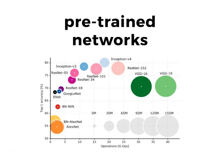

Keras comes with several pre-trained models and easy-to-use examples on how to fine-tune models. You can read more on the documentation.

1.2 What is the Batch Normalization layer?

The Batch Normalization layer was introduced in 2014 by Ioffe and Szegedy. It addresses the vanishing gradient problem by standardizing the output of the previous layer, it speeds up the training by reducing the number of required iterations and it enables the training of deeper neural networks. Explaining exactly how it works is beyond the scope of this post but I strongly encourage you to read the original paper. An oversimplified explanation is that it rescales the input by subtracting its mean and by dividing with its standard deviation; it can also learn to undo the transformation if necessary.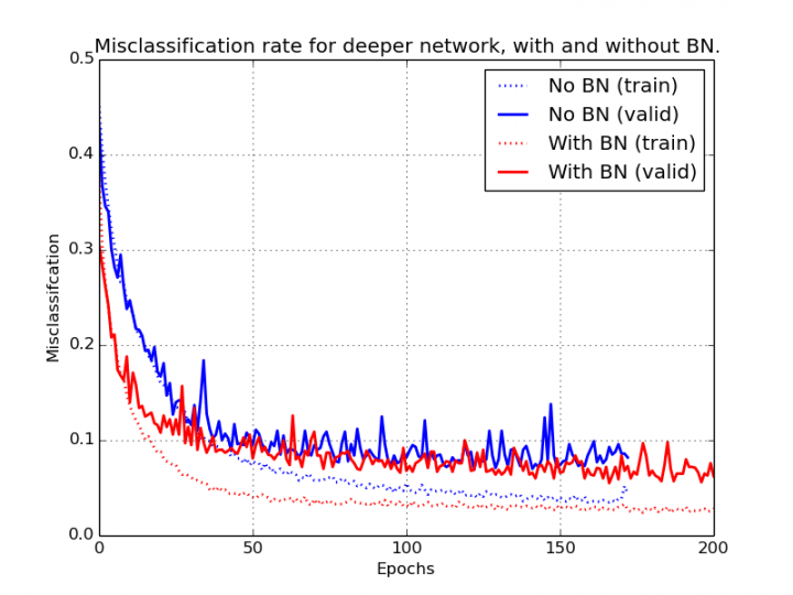

1.3 What is the learning_phase in Keras?

Some layers operate differently during training and inference mode. The most notable examples are the Batch Normalization and the Dropout layers. In the case of BN, during training we use the mean and variance of the mini-batch to rescale the input. On the other hand, during inference we use the moving average and variance that was estimated during training.

Keras knows in which mode to run because it has a built-in mechanism called learning_phase. The learning phase controls whether the network is on train or test mode. If it is not manually set by the user, during fit() the network runs with learning_phase=1 (train mode). While producing predictions (for example when we call the predict() & evaluate() methods or at the validation step of the fit()) the network runs with learning_phase=0 (test mode). Even though it is not recommended, the user is also able to statically change the learning_phase to a specific value but this needs to happen before any model or tensor is added in the graph. If the learning_phase is set statically, Keras will be locked to whichever mode the user selected.

1.4 How did Keras implement Batch Normalization over time?

Keras has changed the behavior of Batch Normalization several times but the most recent significant update happened in Keras 2.1.3. Before v2.1.3 when the BN layer was frozen (trainable = False) it kept updating its batch statistics, something that caused epic headaches to its users.

This was not just a weird policy, it was actually wrong. Imagine that a BN layer exists between convolutions; if the layer is frozen no changes should happen to it. If we do update partially its weights and the next layers are also frozen, they will never get the chance to adjust to the updates of the mini-batch statistics leading to higher error. Thankfully starting from version 2.1.3, when a BN layer is frozen it no longer updates its statistics. But is that enough? Not if you are using Transfer Learning.

Below I describe exactly what is the problem and I sketch out the technical implementation for solving it. I also provide a few examples to show the effects on model’s accuracy before and after the patch is applied.

2.1 Technical description of the problem

The problem with the current implementation of Keras is that when a BN layer is frozen, it continues to use the mini-batch statistics during training. I believe a better approach when the BN is frozen is to use the moving mean and variance that it learned during training. Why? For the same reasons why the mini-batch statistics should not be updated when the layer is frozen: it can lead to poor results because the next layers are not trained properly.

Assume you are building a Computer Vision model but you don’t have enough data, so you decide to use one of the pre-trained CNNs of Keras and fine-tune it. Unfortunately, by doing so you get no guarantees that the mean and variance of your new dataset inside the BN layers will be similar to the ones of the original dataset. Remember that at the moment, during training your network will always use the mini-batch statistics either the BN layer is frozen or not; also during inference you will use the previously learned statistics of the frozen BN layers. As a result, if you fine-tune the top layers, their weights will be adjusted to the mean/variance of the new dataset. Nevertheless, during inference they will receive data which are scaled differently because the mean/variance of the original dataset will be used.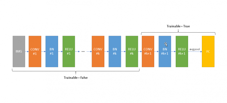

Above I provide a simplistic (and unrealistic) architecture for demonstration purposes. Let’s assume that we fine-tune the model from Convolution k+1 up until the top of the network (right side) and we keep frozen the bottom (left side). During training all BN layers from 1 to k will use the mean/variance of your training data. This will have negative effects on the frozen ReLUs if the mean and variance on each BN are not close to the ones learned during pre-training. It will also cause the rest of the network (from CONV k+1 and later) to be trained with inputs that have different scales comparing to what will receive during inference. During training your network can adapt to these changes, nevertheless the moment you switch to prediction-mode, Keras will use different standardization statistics, something that will swift the distribution of the inputs of the next layers leading to poor results.

2.2 How can you detect if you are affected?

One way to detect it is to set statically the learning phase of Keras to 1 (train mode) and to 0 (test mode) and evaluate your model in each case. If there is significant difference in accuracy on the same dataset, you are being affected by the problem. It’s worth pointing out that, due to the way the learning_phase mechanism is implemented in Keras, it is typically not advised to mess with it. Changes on the learning_phase will have no effect on models that are already compiled and used; as you can see on the examples on the next subsections, the best way to do this is to start with a clean session and change the learning_phase before any tensor is defined in the graph.

Another way to detect the problem while working with binary classifiers is to check the accuracy and the AUC. If the accuracy is close to 50% but the AUC is close to 1 (and also you observe differences between train/test mode on the same dataset), it could be that the probabilities are out-of-scale due the BN statistics. Similarly, for regression you can use MSE and Spearman’s correlation to detect it.

2.3 How can we fix it?

I believe that the problem can be fixed if the frozen BN layers are actually just that: permanently locked in test mode. Implementation-wise, the trainable flag needs to be part of the computational graph and the behavior of the BN needs to depend not only on the learning_phase but also on the value of the trainable property. You can find the details of my implementation on Github.

By applying the above fix, when a BN layer is frozen it will no longer use the mini-batch statistics but instead use the ones learned during training. As a result, there will be no discrepancy between training and test modes which leads to increased accuracy. Obviously when the BN layer is not frozen, it will continue using the mini-batch statistics during training.

2.4 Assessing the effects of the patch

Even though I wrote the above implementation recently, the idea behind it is heavily tested on real-world problems using various workarounds that have the same effect. For example, the discrepancy between training and testing modes and can be avoided by splitting the network in two parts (frozen and unfrozen) and performing cached training (passing data through the frozen model once and then using them to train the unfrozen network). Nevertheless, because the “trust me I’ve done this before” typically bears no weight, below I provide a few examples that show the effects of the new implementation in practice.

Here are a few important points about the experiment:

1. I will use a tiny amount of data to intentionally overfit the model and I will train & validate the model on the same dataset. By doing so, I expect near perfect accuracy and identical performance on the train/validation dataset.
2. If during validation I get significantly lower accuracy on the same dataset, I will have a clear indication that the current BN policy affects negatively the performance of the model during inference.
3. Any preprocessing will take place outside of Generators. This is done to work around a bug that was introduced in v2.1.5 (currently fixed on upcoming v2.1.6 and latest master).
4. We will force Keras to use different learning phases during evaluation. If we spot differences between the reported accuracy we will know we are affected by the current BN policy.

The code for the experiment is shown below:

import numpy as np
from keras.datasets import cifar10
from scipy.misc import imresize

from keras.preprocessing.image import ImageDataGenerator
from keras.applications.resnet50 import ResNet50, preprocess_input
from keras.models import Model, load_model
from keras.layers import Dense, Flatten
from keras import backend as K


seed = 42
epochs = 10
records_per_class = 100

# We take only 2 classes from CIFAR10 and a very small sample to intentionally overfit the model.
# We will also use the same data for train/test and expect that Keras will give the same accuracy.
(x, y), _ = cifar10.load_data()

def filter_resize(category):
   # We do the preprocessing here instead in the Generator to get around a bug on Keras 2.1.5.
   return [preprocess_input(imresize(img, (224,224)).astype('float')) for img in x[y.flatten()==category][:records_per_class]]

x = np.stack(filter_resize(3)+filter_resize(5))
records_per_class = x.shape[0] // 2
y = np.array([[1,0]]*records_per_class + [[0,1]]*records_per_class)


# We will use a pre-trained model and finetune the top layers.
np.random.seed(seed)
base_model = ResNet50(weights='imagenet', include_top=False, input_shape=(224, 224, 3))
l = Flatten()(base_model.output)
predictions = Dense(2, activation='softmax')(l)
model = Model(inputs=base_model.input, outputs=predictions)

for layer in model.layers[:140]:
   layer.trainable = False

for layer in model.layers[140:]:
   layer.trainable = True

model.compile(optimizer='sgd', loss='categorical_crossentropy', metrics=['accuracy'])
model.fit_generator(ImageDataGenerator().flow(x, y, seed=42), epochs=epochs, validation_data=ImageDataGenerator().flow(x, y, seed=42))

# Store the model on disk
model.save('tmp.h5')


# In every test we will clear the session and reload the model to force Learning_Phase values to change.
print('DYNAMIC LEARNING_PHASE')
K.clear_session()
model = load_model('tmp.h5')
# This accuracy should match exactly the one of the validation set on the last iteration.
print(model.evaluate_generator(ImageDataGenerator().flow(x, y, seed=42)))


print('STATIC LEARNING_PHASE = 0')
K.clear_session()
K.set_learning_phase(0)
model = load_model('tmp.h5')
# Again the accuracy should match the above.
print(model.evaluate_generator(ImageDataGenerator().flow(x, y, seed=42)))


print('STATIC LEARNING_PHASE = 1')
K.clear_session()
K.set_learning_phase(1)
model = load_model('tmp.h5')
# The accuracy will be close to the one of the training set on the last iteration.
print(model.evaluate_generator(ImageDataGenerator().flow(x, y, seed=42)))

Let’s check the results on Keras v2.1.5:

Epoch 1/10
1/7 [===>..........................] - ETA: 25s - loss: 0.8751 - acc: 0.5312
2/7 [=======>......................] - ETA: 11s - loss: 0.8594 - acc: 0.4531
3/7 [===========>..................] - ETA: 7s - loss: 0.8398 - acc: 0.4688 
4/7 [================>.............] - ETA: 4s - loss: 0.8467 - acc: 0.4844
5/7 [====================>.........] - ETA: 2s - loss: 0.7904 - acc: 0.5437
6/7 [========================>.....] - ETA: 1s - loss: 0.7593 - acc: 0.5625
7/7 [==============================] - 12s 2s/step - loss: 0.7536 - acc: 0.5744 - val_loss: 0.6526 - val_acc: 0.6650

Epoch 2/10
1/7 [===>..........................] - ETA: 4s - loss: 0.3881 - acc: 0.8125
2/7 [=======>......................] - ETA: 3s - loss: 0.3945 - acc: 0.7812
3/7 [===========>..................] - ETA: 2s - loss: 0.3956 - acc: 0.8229
4/7 [================>.............] - ETA: 1s - loss: 0.4223 - acc: 0.8047
5/7 [====================>.........] - ETA: 1s - loss: 0.4483 - acc: 0.7812
6/7 [========================>.....] - ETA: 0s - loss: 0.4325 - acc: 0.7917
7/7 [==============================] - 8s 1s/step - loss: 0.4095 - acc: 0.8089 - val_loss: 0.4722 - val_acc: 0.7700

Epoch 3/10
1/7 [===>..........................] - ETA: 4s - loss: 0.2246 - acc: 0.9375
2/7 [=======>......................] - ETA: 3s - loss: 0.2167 - acc: 0.9375
3/7 [===========>..................] - ETA: 2s - loss: 0.2260 - acc: 0.9479
4/7 [================>.............] - ETA: 2s - loss: 0.2179 - acc: 0.9375
5/7 [====================>.........] - ETA: 1s - loss: 0.2356 - acc: 0.9313
6/7 [========================>.....] - ETA: 0s - loss: 0.2392 - acc: 0.9427
7/7 [==============================] - 8s 1s/step - loss: 0.2288 - acc: 0.9456 - val_loss: 0.4282 - val_acc: 0.7800

Epoch 4/10
1/7 [===>..........................] - ETA: 4s - loss: 0.2183 - acc: 0.9688
2/7 [=======>......................] - ETA: 3s - loss: 0.1899 - acc: 0.9844
3/7 [===========>..................] - ETA: 2s - loss: 0.1887 - acc: 0.9792
4/7 [================>.............] - ETA: 1s - loss: 0.1995 - acc: 0.9531
5/7 [====================>.........] - ETA: 1s - loss: 0.1932 - acc: 0.9625
6/7 [========================>.....] - ETA: 0s - loss: 0.1819 - acc: 0.9688
7/7 [==============================] - 8s 1s/step - loss: 0.1743 - acc: 0.9747 - val_loss: 0.3778 - val_acc: 0.8400

Epoch 5/10
1/7 [===>..........................] - ETA: 3s - loss: 0.0973 - acc: 1.0000
2/7 [=======>......................] - ETA: 3s - loss: 0.0828 - acc: 1.0000
3/7 [===========>..................] - ETA: 2s - loss: 0.0851 - acc: 1.0000
4/7 [================>.............] - ETA: 1s - loss: 0.0897 - acc: 1.0000
5/7 [====================>.........] - ETA: 1s - loss: 0.0928 - acc: 1.0000
6/7 [========================>.....] - ETA: 0s - loss: 0.0936 - acc: 1.0000
7/7 [==============================] - 8s 1s/step - loss: 0.1337 - acc: 0.9838 - val_loss: 0.3916 - val_acc: 0.8100

Epoch 6/10
1/7 [===>..........................] - ETA: 4s - loss: 0.0747 - acc: 1.0000
2/7 [=======>......................] - ETA: 3s - loss: 0.0852 - acc: 1.0000
3/7 [===========>..................] - ETA: 2s - loss: 0.0812 - acc: 1.0000
4/7 [================>.............] - ETA: 1s - loss: 0.0831 - acc: 1.0000
5/7 [====================>.........] - ETA: 1s - loss: 0.0779 - acc: 1.0000
6/7 [========================>.....] - ETA: 0s - loss: 0.0766 - acc: 1.0000
7/7 [==============================] - 8s 1s/step - loss: 0.0813 - acc: 1.0000 - val_loss: 0.3637 - val_acc: 0.8550

Epoch 7/10
1/7 [===>..........................] - ETA: 1s - loss: 0.2478 - acc: 0.8750
2/7 [=======>......................] - ETA: 2s - loss: 0.1966 - acc: 0.9375
3/7 [===========>..................] - ETA: 2s - loss: 0.1528 - acc: 0.9583
4/7 [================>.............] - ETA: 1s - loss: 0.1300 - acc: 0.9688
5/7 [====================>.........] - ETA: 1s - loss: 0.1193 - acc: 0.9750
6/7 [========================>.....] - ETA: 0s - loss: 0.1196 - acc: 0.9792
7/7 [==============================] - 8s 1s/step - loss: 0.1084 - acc: 0.9838 - val_loss: 0.3546 - val_acc: 0.8600

Epoch 8/10
1/7 [===>..........................] - ETA: 4s - loss: 0.0539 - acc: 1.0000
2/7 [=======>......................] - ETA: 2s - loss: 0.0900 - acc: 1.0000
3/7 [===========>..................] - ETA: 2s - loss: 0.0815 - acc: 1.0000
4/7 [================>.............] - ETA: 1s - loss: 0.0740 - acc: 1.0000
5/7 [====================>.........] - ETA: 1s - loss: 0.0700 - acc: 1.0000
6/7 [========================>.....] - ETA: 0s - loss: 0.0701 - acc: 1.0000
7/7 [==============================] - 8s 1s/step - loss: 0.0695 - acc: 1.0000 - val_loss: 0.3269 - val_acc: 0.8600

Epoch 9/10
1/7 [===>..........................] - ETA: 4s - loss: 0.0306 - acc: 1.0000
2/7 [=======>......................] - ETA: 3s - loss: 0.0377 - acc: 1.0000
3/7 [===========>..................] - ETA: 2s - loss: 0.0898 - acc: 0.9583
4/7 [================>.............] - ETA: 1s - loss: 0.0773 - acc: 0.9688
5/7 [====================>.........] - ETA: 1s - loss: 0.0742 - acc: 0.9750
6/7 [========================>.....] - ETA: 0s - loss: 0.0708 - acc: 0.9792
7/7 [==============================] - 8s 1s/step - loss: 0.0659 - acc: 0.9838 - val_loss: 0.3604 - val_acc: 0.8600

Epoch 10/10
1/7 [===>..........................] - ETA: 3s - loss: 0.0354 - acc: 1.0000
2/7 [=======>......................] - ETA: 3s - loss: 0.0381 - acc: 1.0000
3/7 [===========>..................] - ETA: 2s - loss: 0.0354 - acc: 1.0000
4/7 [================>.............] - ETA: 1s - loss: 0.0828 - acc: 0.9688
5/7 [====================>.........] - ETA: 1s - loss: 0.0791 - acc: 0.9750
6/7 [========================>.....] - ETA: 0s - loss: 0.0794 - acc: 0.9792
7/7 [==============================] - 8s 1s/step - loss: 0.0704 - acc: 0.9838 - val_loss: 0.3615 - val_acc: 0.8600

DYNAMIC LEARNING_PHASE
[0.3614931714534759, 0.86]

STATIC LEARNING_PHASE = 0
[0.3614931714534759, 0.86]

STATIC LEARNING_PHASE = 1
[0.025861846953630446, 1.0]

As we can see above, during training the model learns very well the data and achieves on the training set near-perfect accuracy. Still at the end of each iteration, while evaluating the model on the same dataset, we get significant differences in loss and accuracy. Note that we should not be getting this; we have overfitted intentionally the model on the specific dataset and the training/validation datasets are identical.

After the training is completed we evaluate the model using 3 different learning_phase configurations: Dynamic, Static = 0 (test mode) and Static = 1 (training mode). As we can see the first two configurations will provide identical results in terms of loss and accuracy and their value matches the reported accuracy of the model on the validation set in the last iteration. Nevertheless, once we switch to training mode, we observe a massive discrepancy (improvement).  Why it that? As we said earlier, the weights of the network are tuned expecting to receive data scaled with the mean/variance of the training data. Unfortunately, those statistics are different from the ones stored in the BN layers. Since the BN layers were frozen, these statistics were never updated. This discrepancy between the values of the BN statistics leads to the deterioration of the accuracy during inference.

Let’s see what happens once we apply the patch:

Epoch 1/10
1/7 [===>..........................] - ETA: 26s - loss: 0.9992 - acc: 0.4375
2/7 [=======>......................] - ETA: 12s - loss: 1.0534 - acc: 0.4375
3/7 [===========>..................] - ETA: 7s - loss: 1.0592 - acc: 0.4479 
4/7 [================>.............] - ETA: 4s - loss: 0.9618 - acc: 0.5000
5/7 [====================>.........] - ETA: 2s - loss: 0.8933 - acc: 0.5250
6/7 [========================>.....] - ETA: 1s - loss: 0.8638 - acc: 0.5417
7/7 [==============================] - 13s 2s/step - loss: 0.8357 - acc: 0.5570 - val_loss: 0.2414 - val_acc: 0.9450

Epoch 2/10
1/7 [===>..........................] - ETA: 4s - loss: 0.2331 - acc: 0.9688
2/7 [=======>......................] - ETA: 2s - loss: 0.3308 - acc: 0.8594
3/7 [===========>..................] - ETA: 2s - loss: 0.3986 - acc: 0.8125
4/7 [================>.............] - ETA: 1s - loss: 0.3721 - acc: 0.8281
5/7 [====================>.........] - ETA: 1s - loss: 0.3449 - acc: 0.8438
6/7 [========================>.....] - ETA: 0s - loss: 0.3168 - acc: 0.8646
7/7 [==============================] - 9s 1s/step - loss: 0.3165 - acc: 0.8633 - val_loss: 0.1167 - val_acc: 0.9950

Epoch 3/10
1/7 [===>..........................] - ETA: 1s - loss: 0.2457 - acc: 1.0000
2/7 [=======>......................] - ETA: 2s - loss: 0.2592 - acc: 0.9688
3/7 [===========>..................] - ETA: 2s - loss: 0.2173 - acc: 0.9688
4/7 [================>.............] - ETA: 1s - loss: 0.2122 - acc: 0.9688
5/7 [====================>.........] - ETA: 1s - loss: 0.2003 - acc: 0.9688
6/7 [========================>.....] - ETA: 0s - loss: 0.1896 - acc: 0.9740
7/7 [==============================] - 9s 1s/step - loss: 0.1835 - acc: 0.9773 - val_loss: 0.0678 - val_acc: 1.0000

Epoch 4/10
1/7 [===>..........................] - ETA: 1s - loss: 0.2051 - acc: 1.0000
2/7 [=======>......................] - ETA: 2s - loss: 0.1652 - acc: 0.9844
3/7 [===========>..................] - ETA: 2s - loss: 0.1423 - acc: 0.9896
4/7 [================>.............] - ETA: 1s - loss: 0.1289 - acc: 0.9922
5/7 [====================>.........] - ETA: 1s - loss: 0.1225 - acc: 0.9938
6/7 [========================>.....] - ETA: 0s - loss: 0.1149 - acc: 0.9948
7/7 [==============================] - 9s 1s/step - loss: 0.1060 - acc: 0.9955 - val_loss: 0.0455 - val_acc: 1.0000

Epoch 5/10
1/7 [===>..........................] - ETA: 4s - loss: 0.0769 - acc: 1.0000
2/7 [=======>......................] - ETA: 2s - loss: 0.0846 - acc: 1.0000
3/7 [===========>..................] - ETA: 2s - loss: 0.0797 - acc: 1.0000
4/7 [================>.............] - ETA: 1s - loss: 0.0736 - acc: 1.0000
5/7 [====================>.........] - ETA: 1s - loss: 0.0914 - acc: 1.0000
6/7 [========================>.....] - ETA: 0s - loss: 0.0858 - acc: 1.0000
7/7 [==============================] - 9s 1s/step - loss: 0.0808 - acc: 1.0000 - val_loss: 0.0346 - val_acc: 1.0000

Epoch 6/10
1/7 [===>..........................] - ETA: 1s - loss: 0.1267 - acc: 1.0000
2/7 [=======>......................] - ETA: 2s - loss: 0.1039 - acc: 1.0000
3/7 [===========>..................] - ETA: 2s - loss: 0.0893 - acc: 1.0000
4/7 [================>.............] - ETA: 1s - loss: 0.0780 - acc: 1.0000
5/7 [====================>.........] - ETA: 1s - loss: 0.0758 - acc: 1.0000
6/7 [========================>.....] - ETA: 0s - loss: 0.0789 - acc: 1.0000
7/7 [==============================] - 9s 1s/step - loss: 0.0738 - acc: 1.0000 - val_loss: 0.0248 - val_acc: 1.0000

Epoch 7/10
1/7 [===>..........................] - ETA: 4s - loss: 0.0344 - acc: 1.0000
2/7 [=======>......................] - ETA: 3s - loss: 0.0385 - acc: 1.0000
3/7 [===========>..................] - ETA: 3s - loss: 0.0467 - acc: 1.0000
4/7 [================>.............] - ETA: 1s - loss: 0.0445 - acc: 1.0000
5/7 [====================>.........] - ETA: 1s - loss: 0.0446 - acc: 1.0000
6/7 [========================>.....] - ETA: 0s - loss: 0.0429 - acc: 1.0000
7/7 [==============================] - 9s 1s/step - loss: 0.0421 - acc: 1.0000 - val_loss: 0.0202 - val_acc: 1.0000

Epoch 8/10
1/7 [===>..........................] - ETA: 4s - loss: 0.0319 - acc: 1.0000
2/7 [=======>......................] - ETA: 3s - loss: 0.0300 - acc: 1.0000
3/7 [===========>..................] - ETA: 3s - loss: 0.0320 - acc: 1.0000
4/7 [================>.............] - ETA: 2s - loss: 0.0307 - acc: 1.0000
5/7 [====================>.........] - ETA: 1s - loss: 0.0303 - acc: 1.0000
6/7 [========================>.....] - ETA: 0s - loss: 0.0291 - acc: 1.0000
7/7 [==============================] - 9s 1s/step - loss: 0.0358 - acc: 1.0000 - val_loss: 0.0167 - val_acc: 1.0000

Epoch 9/10
1/7 [===>..........................] - ETA: 4s - loss: 0.0246 - acc: 1.0000
2/7 [=======>......................] - ETA: 3s - loss: 0.0255 - acc: 1.0000
3/7 [===========>..................] - ETA: 3s - loss: 0.0258 - acc: 1.0000
4/7 [================>.............] - ETA: 2s - loss: 0.0250 - acc: 1.0000
5/7 [====================>.........] - ETA: 1s - loss: 0.0252 - acc: 1.0000
6/7 [========================>.....] - ETA: 0s - loss: 0.0260 - acc: 1.0000
7/7 [==============================] - 9s 1s/step - loss: 0.0327 - acc: 1.0000 - val_loss: 0.0143 - val_acc: 1.0000

Epoch 10/10
1/7 [===>..........................] - ETA: 4s - loss: 0.0251 - acc: 1.0000
2/7 [=======>......................] - ETA: 2s - loss: 0.0228 - acc: 1.0000
3/7 [===========>..................] - ETA: 2s - loss: 0.0217 - acc: 1.0000
4/7 [================>.............] - ETA: 1s - loss: 0.0249 - acc: 1.0000
5/7 [====================>.........] - ETA: 1s - loss: 0.0244 - acc: 1.0000
6/7 [========================>.....] - ETA: 0s - loss: 0.0239 - acc: 1.0000
7/7 [==============================] - 9s 1s/step - loss: 0.0290 - acc: 1.0000 - val_loss: 0.0127 - val_acc: 1.0000

DYNAMIC LEARNING_PHASE
[0.012697912137955427, 1.0]

STATIC LEARNING_PHASE = 0
[0.012697912137955427, 1.0]

STATIC LEARNING_PHASE = 1
[0.01744014158844948, 1.0]

First of all, we observe that the network converges significantly faster and achieves perfect accuracy. We also see that there is no longer a discrepancy in terms of accuracy when we switch between different learning_phase values.

2.5 How does the patch perform on a real dataset?

So how does the patch perform on a more realistic experiment? Let’s use Keras’ pre-trained ResNet50 (originally fit on imagenet), remove the top classification layer and fine-tune it with and without the patch and compare the results. For data, we will use CIFAR10 (the standard train/test split provided by Keras) and we will resize the images to 224×224 to make them compatible with the ResNet50’s input size.

We will do 10 epochs to train the top classification layer using RSMprop and then we will do another 5 to fine-tune everything after the 139th layer using SGD(lr=1e-4, momentum=0.9). Without the patch our model achieves an accuracy of 87.44%. Using the patch, we get an accuracy of 92.36%, almost 5 points higher.

2.6 Should we apply the same fix to other layers such as Dropout?

Batch Normalization is not the only layer that operates differently between train and test modes. Dropout and its variants also have the same effect. Should we apply the same policy to all these layers? I believe not (even though I would love to hear your thoughts on this). The reason is that Dropout is used to avoid overfitting, thus locking it permanently to prediction mode during training would defeat its purpose. What do you think?

I strongly believe that this discrepancy must be solved in Keras. I’ve seen even more profound effects (from 100% down to 50% accuracy) in real-world applications caused by this problem. I plan to send already sent a PR to Keras with the fix and hopefully it will be accepted.

If you liked this blogpost, please take a moment to share it on Facebook or Twitter. 🙂